
A short article on the simpleITK library’s handling of image data. After this, you’d have a good general understanding of the basic concepts regarding Image handling in SimpleITK
What is SimpleITK?
SimpleITK (SITK) is a simplified programming interface to the algorithms and data structures of the Insight Toolkit (ITK). It was developed at the National Institutes of Health (NIH) as an open resource, its primary goal is to make the algorithms available in the ITK library accessible to the broadest range of scientists whose work includes image analysis. The library is available in a wide variety of languages, these are C++, Python, R, Java, C#, Lua, Ruby, and Tcl.

The toolkit is organized around a data-flow architecture. That is, data is represented using data objects which are in turn processed by process objects (filters). Data objects and process objects are connected together into pipelines. Pipelines are capable of processing the data in pieces according to a user-specified memory limit set on the pipeline. However, the toolkit does not address visualization or a graphical user interface. These are left to other toolkits
Images in SimpleITK
Images in SITK are different from those we are used to seeing every day. Each pixel or voxel [3D pixel basically] is not isotropically spaced. The image is defined as a physical entity in 3D space. That means, that not only does each pixel have coordinates, but there are also direction vectors for the axis as well. Simply put, this means,
- Images can have different spacing between pixels along each axis
- The axes are not necessarily orthogonal.
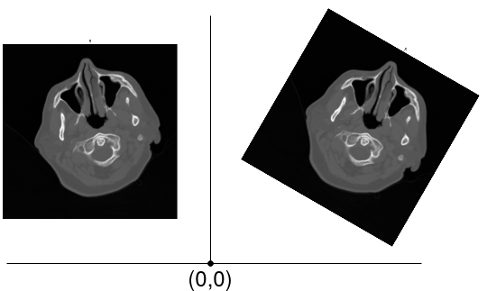
But what will happen if we use something like NumPy to read the image data and directly plot it instead?

Left. Image displayed with a viewer that is not aware of spatial meta-data. Right. Image displayed with a viewer that is aware of spatial meta- data. Image authors: here
As visible, without spatial information, scans with anisotropic spacing between pixels, as shown above, will seem distorted. Now that we’ve got a general idea of these images, let’s jump into the specifics.
Loading an image
Before we can analyze an image, we need to load it into memory.
image = sitk.ReadImage("/path/to/image/image.dcm")
print("Type:", type(image), "Image size:", size[0], size[1], size[2])
Outputs
Type: <class 'SimpleITK.SimpleITK.Image'> Image size: 512 512 3
Or if you wish to load an entire series all at once
reader = sitk.ImageSeriesReader()
dicom_names = reader.GetGDCMSeriesFileNames("/path/to/series/directory")
reader.SetFileNames(dicom_names)

image_series = reader.Execute()
size = image_series.GetSize()
print("Type:", type(image_series), "Image size:", size[0], size[1], size[2])
Outputs
Type: <class 'SimpleITK.SimpleITK.Image'> Image size: 512 512 42
A series will be loaded as a 3D image/array. If you wish to access any particular pixel values simply use the following format. For slicing, replace the indices accordingly in the general pythonic format.
## .. code to get image

x = 10  # X-coordinate of the pixel
y = 10  # Y-coordinate of the pixel
z = 0   # Z-coordinate of the pixel
value = image.GetPixel(
    (x, y, z)
)  # May throw error if (x,y,z) is out of bounds of the physical space of the image.
value2 = image[x, y, z]  # Another way of accessing value

print("image.GetPixel((x,y,z)) = ", value)
print("image[x,y,z] = ", value2)
Outputs
image.GetPixel((x,y,z)) = 123
image[x,y,z] = 123
This will give us an object of SITK Image class. Now how do we view it? The recommended viewing library from SITK is FIJI. You can, however, also use Matplotlib to view 2D images.
## .. code to get the image

## If you already have FIJI installed
sitk.show(image, "Title")

## Using matplotlib instead
nd_image = sitk.GetArrayViewFromImage(image)
nd_image = np.squeeze(
    nd_image
)  # plt cannot plot (1,x,x) it needs to be (x,x) for a 2D image
plt.imshow(nd_image, cmap="gray")
print(f"Image shape {nd_image.shape}")
Outputs
Image shape (512,512)
Do Note: The array from sitk.GetArrayViewFromImage(image), has its shape in the Channels first format, this means it is indexed as (z_index, y_index, x_index) while in the indexing example above, we’ve seen that an SITK image size is in Channels last format, which means it is indexed as (x_index, y_index, z_index)
Image attributes
Now, let’s get into the details of the attributes of these images
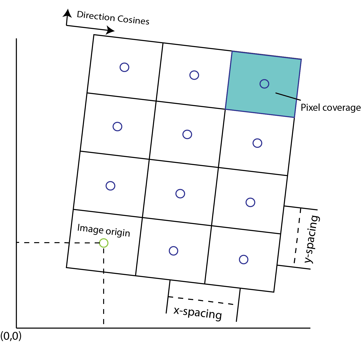
Anatomy of an SITK image. Explanations for each attribute mentioned below
-
Origin: This is the starting point of the image. Identified by the left-bottom corner of the image as shown in the figure. Use
image.GetOrigin()to get the spacing of an SITK image. To change the origin of an image, read the transforms section. This attribute is crucial when composing 2 images on top of each other. If their origins do not match, SITK does not allow the super-position of 2 images. -
Spacing: This is the distance between pixels along each of the dimensions. The picture below shows two images with different spacing values. As you can see, image stretching can be performed by changing this value. Use
image.GetSpacing()to get the spacing of an SITK image. -
Size: This defines the number of pixels in each dimension of the image. Use
image.GetSize()to get the size of an SITK image. -
Direction Cosines: The direction in which pixel intensities are mentioned in the image array. Direction cosines define the axis of the image beginning from the image origin. Defined by a tuple containing n*n flattened values of n-dimensional vectors along each axis in a sequential order, where n is the dimensionality of the image. For eg. the 2D image above has direction cosines approximately (0.9805, -0.1961, -0.1961, 0.9805). Use
image.GetDirection()to get the spacing of the SITK image.
While these two images look the same to our eye. For SITK these are not equivalent. Consider the marked middle point to be (0,0) in physical space. Then both these images have a different origin, and direction cosines. So even though they have the same spacing and size, contrary to general belief, they're not equivalent. Image authors: here
Transforms
Spatial transformations in SITK convert a point x to T(x) in the following way (except for translation transform)
T(x) = A(x-c) + t + c
Here,
- Matrix: the matrix A
- Center: the point c
- Translation: the vector t
- Offset: t + c - Ac
Translations can be applied directly to points in SITK. The code below performs simple translation on a point in 3D space.
dimension = 2
offset = [1, 2]

translation = sitk.TranslationTransform(dimension, offset)

point = [10, 10]
transformed_point = translation.TransformPoint(point)
translation_inverse = translation.GetInverse()

print(translation)
print(
    "original point: {}\ntransformed point: {}\nback to original: {}".format(
        point, transformed_point, translation_inverse.TransformPoint(transformed_point)
    )
)
Outputs
itk::simple::TranslationTransform
 TranslationTransform (0x2a4ed90)
   RTTI typeinfo:   itk::TranslationTransform<double, 2u>
   Reference Count: 1
   Modified Time: 666
   Debug: Off
   Object Name:
   Observers:
     none
   Offset: [1, 2]
original point: [10, 10]
transformed point: (11.0, 12.0)
back to original: (10.0, 10.0)

Translation transform. Circle: Original point. Triangle: Shifted point
Some common transforms
Translation: Simply moving a point from one place to another. y = x + t
translation = sitk.TranslationTransform(dimension, offset)
Euler Transforms: This transform applies a rotation and translation to the space given Euler angles and a translation. May be 2D or 3D. Rotation is about a user-specified center.
euler2d = sitk.Euler2DTransform(centre, angle, offset)euler3d = sitk.Euler3DTransform(centre, angleX, angleY, angleZ, translation)
Affine Transforms: An affine transformation is defined mathematically as a linear transformation plus a constant offset. If A is a constant n x n matrix and b is a constant n-vector, then y = Ax+b defines an affine transformation from the n-vector x to the n-vector y.
affine = sitk.AffineTransform(matrix.flatten(), translation, centre)
Resampling
We have applied transforms to points. When we do the same for an entire image, it is termed as resampling in SITK.
## Define translation transform
dimension = 2
offset = (3, 4)
translation = sitk.TranslationTransform(dimension, offset)

## Create a sample grid for demonstration
grid = sitk.GridSource(
    outputPixelType=sitk.sitkUInt16,
    size=(250, 250),
    sigma=(0.5, 0.5),
    gridSpacing=(5.0, 5.0),
    gridOffset=(0.0, 0.0),
    spacing=(0.2, 0.2),
)

## Show the original image
plt.imshow(sitk.GetArrayViewFromImage(grid), cmap="gray", origin="lower")
plt.show()

## Get resampled image and show
resampled = sitk.Resample(grid, translation)
plt.imshow(sitk.GetArrayViewFromImage(resampled), cmap="gray", origin="lower")
plt.show()
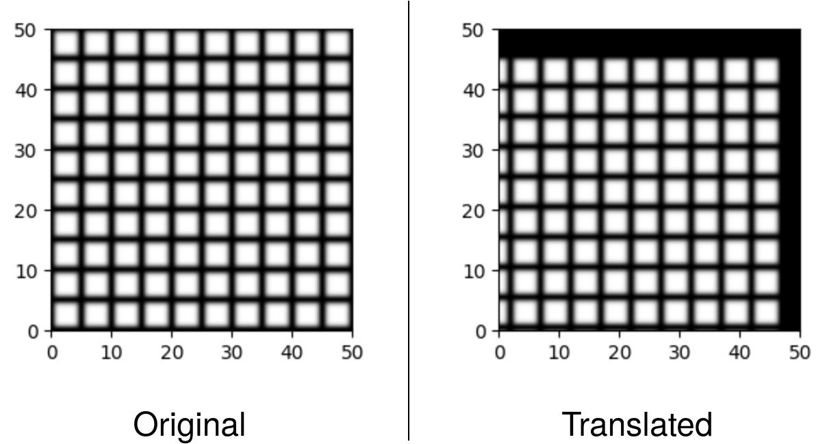
Left. Our original grid image. Right. Grid image after applying translation. Notice how our translation is positive (3,4) but our image moved towards the left and bottom. This is because, translation is defined from output points to input points. i.e (0,0) of output image is mapped to (3,4) of input image. Therefore, the image translates opposite to our expectation
Likewise, if we apply Euler transforms on an image
## Define image to be transformed
grid = sitk.GridSource(
    outputPixelType=sitk.sitkUInt16,
    size=(250, 250),
    sigma=(0.5, 0.5),
    gridSpacing=(5.0, 5.0),
    gridOffset=(0.0, 0.0),
    spacing=(0.2, 0.2),
)

## Define transform
angle = np.pi / 4
offset = (0, 0)
centre = grid.TransformContinuousIndexToPhysicalPoint(np.array(grid.GetSize()) / 2.0)
euler2d = sitk.Euler2DTransform(centre, angle, offset)

## Resample
resampled = sitk.Resample(grid, euler2d)

## Show
plt.imshow(sitk.GetArrayViewFromImage(grid), cmap="gray", origin="lower")
plt.show()
plt.imshow(sitk.GetArrayViewFromImage(resampled), cmap="gray", origin="lower")
plt.show()
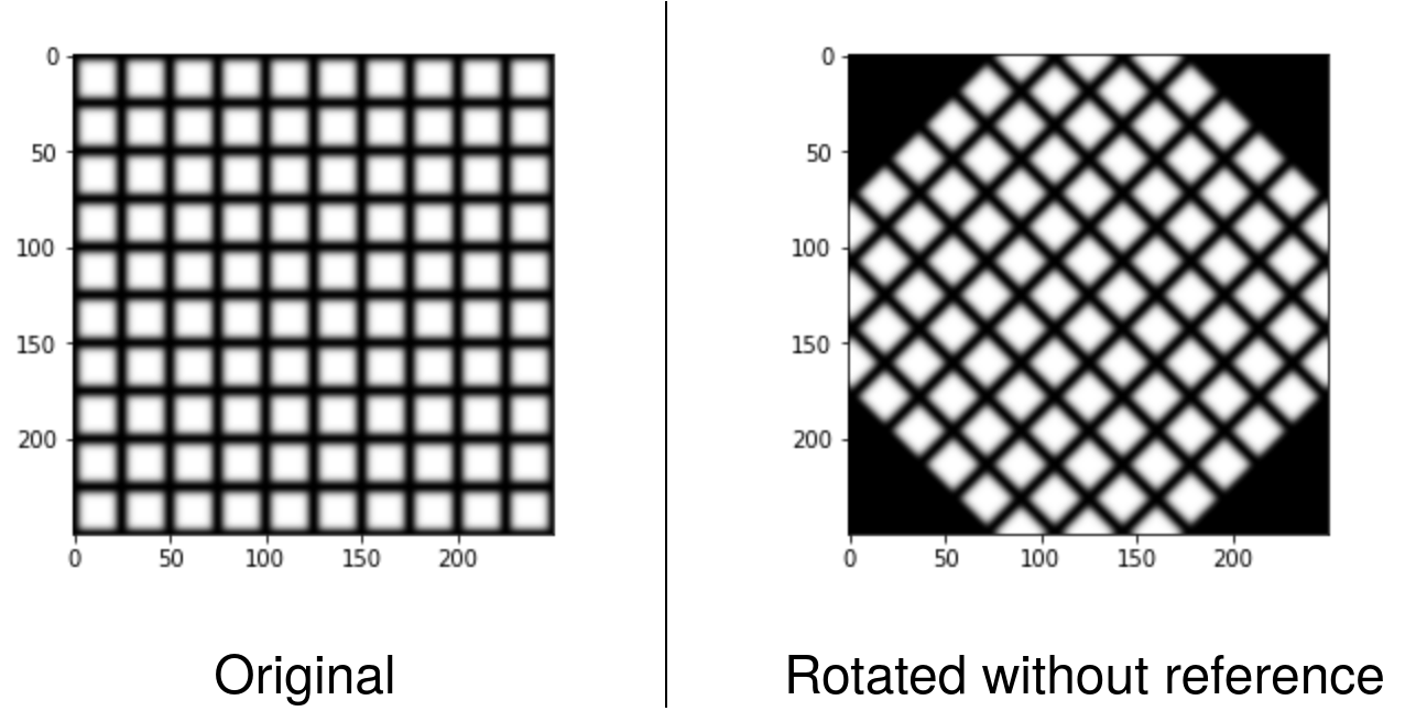
Left. Our original grid image. Right. Grid image after applying rotation of pi/4
In the examples above we did not specify a separate reference image for our mapping. As a result, the resulting image contained black pixels for pixels that were mapped outside the spatial domain of the original image and a partial view of the original image.
If we want the resulting image to contain all of the original image no matter the transformation, we will need to define the resampling grid using our knowledge of the original image’s spatial domain and the inverse of the given transformation.
## Get the grid
grid = sitk.GridSource(
    outputPixelType=sitk.sitkUInt16,
    size=(250, 250),
    sigma=(0.5, 0.5),
    gridSpacing=(5.0, 5.0),
    gridOffset=(0.0, 0.0),
    spacing=(0.2, 0.2),
)

## Define Euler transform and its inverse
angle = np.pi / 4
offset = (0, 0)
centre = grid.TransformContinuousIndexToPhysicalPoint(np.array(grid.GetSize()) / 2.0)
euler2d = sitk.Euler2DTransform(centre, angle, offset)
inv_euler2d = euler2d.GetInverse()

## Make a list of extreme points of our grid
extreme_points = [
    grid.TransformIndexToPhysicalPoint((0, 0)),
    grid.TransformIndexToPhysicalPoint((grid.GetWidth(), 0)),
    grid.TransformIndexToPhysicalPoint((grid.GetWidth(), grid.GetHeight())),
    grid.TransformIndexToPhysicalPoint((0, grid.GetHeight())),
]

## Get a list of the transformed extreme points
extreme_points_transformed = [inv_euler2d.TransformPoint(pnt) for pnt in extreme_points]

## Since we know that the transformed grid's extreme points will also be
## the same as the original's (property of Euler Transform)
## We can determine the extremities of the new image
min_x = min(extreme_points_transformed)[0]
max_x = max(extreme_points_transformed)[0]
min_y = min(extreme_points_transformed, key=lambda p: p[1])[1]
max_y = max(extreme_points_transformed, key=lambda p: p[1])[1]

## Using these new extremities, we can essentially ask SITK to
## map the transform on a bigger canvas
output_spacing = grid.GetSpacing()
output_direction = [1.0, 0.0, 0.0, 1.0]
output_origin = [min_x, min_y]
output_size = [
    int((max_x - min_x) / output_spacing[0]),
    int((max_y - min_y) / output_spacing[1]),
]

## Create the resampled image. We use the sitkLinear function for interpolation.
resampled_image = sitk.Resample(
    grid,
    output_size,
    euler2d,
    sitk.sitkLinear,
    output_origin,
    output_spacing,
    output_direction,
)

## Display new image
plt.imshow(sitk.GetArrayViewFromImage(resampled_image), cmap="gray")
plt.axis("off")
plt.show()
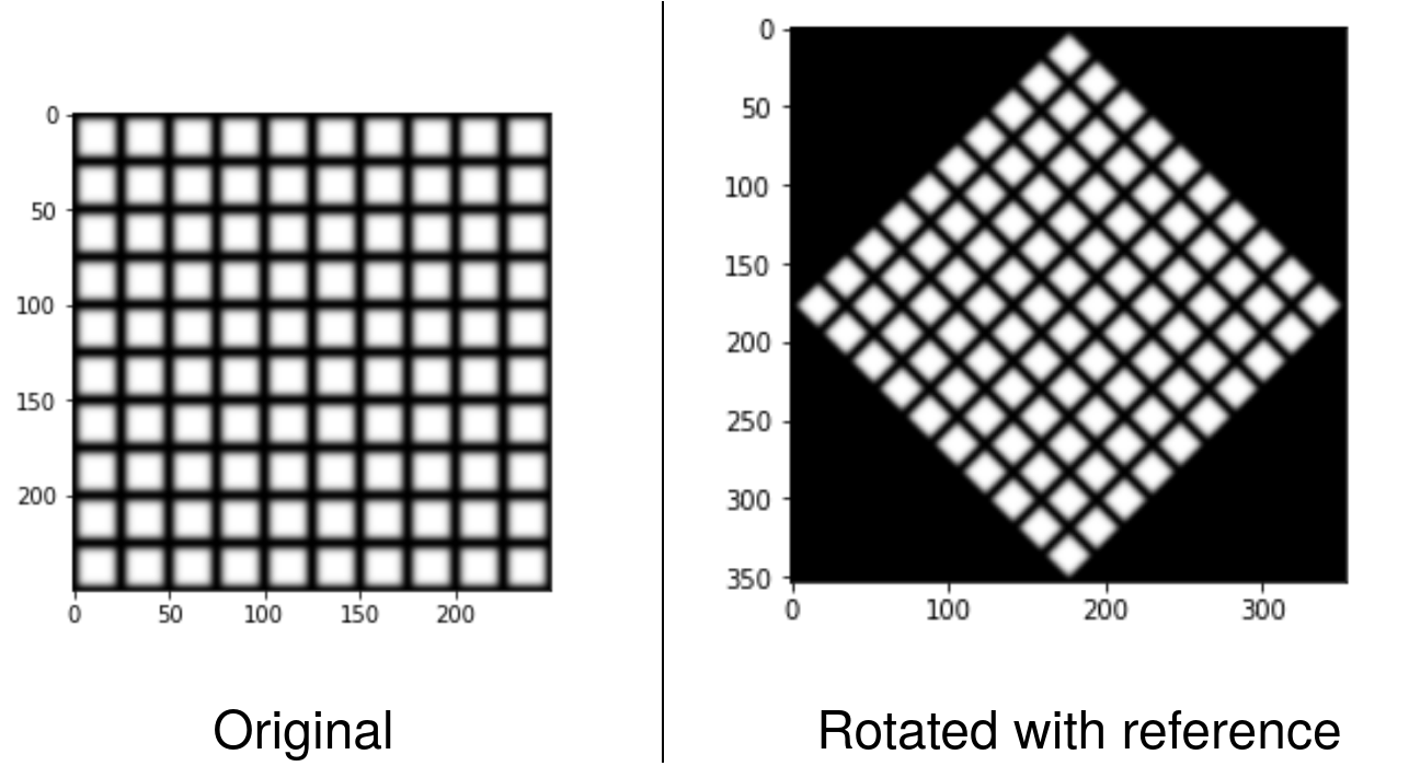
Left. Our original grid image. Right. Grid image after applying rotation with output calculations to account for clipping of the image.
In the above example, we used 4 parameters to define the output image dimensions. SITK provides an easy way for us to bundle all this information into one object called the reference_image
## ..same code as above, till calculation of extremities

## Defining the reference image
reference_image = sitk.Image(
    [
        int((max_x - min_x) / output_spacing[0]),
        int((max_y - min_y) / output_spacing[1]),
    ],
    grid.GetPixelIDValue(),
)
reference_image.SetOrigin([min_x, min_y])
reference_image.SetSpacing(grid.GetSpacing())
reference_image.SetDirection([1.0, 0.0, 0.0, 1.0])

## rRsampling
resampled_image = sitk.Resample(grid, reference_image, euler2d, sitk.sitkLinear)

## Display
plt.imshow(sitk.GetArrayViewFromImage(resampled_image), cmap="gray")
plt.axis("off")
plt.show()

## Reuse the reference_image in other places
This way, the code is smaller and better encapsulated.